


Quantum Chaos on a Quantum Computer with few lines of code


Quantum Chaos
Classical chaotic dynamics is marked by sensitivity to initial conditions: two trajectories that start arbitrarily close in phase space typically separate exponentially fast under time evolution. This exponential divergence is closely tied to mixing and rapid information spreading.
Defining quantum chaos is more subtle. In a broad sense, it refers to quantum dynamics that exhibit “chaotic” hallmarks, such as rapid information scrambling and random-matrix-like features. When a quantum system has a clear classical limit, the question becomes more specific: which dynamical signatures of classical chaos remain meaningful after quantization, and what new interference-driven phenomena appear? Quantum maps offer a particularly clean and widely used setting to explore this connection.
Quantum maps
Classical maps are discrete-time dynamical rules that update a system’s coordinates from one step to the next (e.g., x(t) → x(t+1)), Similarly, quantum maps are discrete-time quantum evolutions, often obtained by quantizing classical maps. A typical example describes free evolution periodically kicked by a position-dependent potential.
Despite their simple definition, they capture key phenomena of quantum chaos, including rapid entanglement growth and interference-driven localization, and often provide insights that carry over to more realistic systems. In 1979, Casati, Chirikov, Izrailev, and Ford identified dynamical localization in kicked chaotic systems, where quantum interference suppresses classical diffusion. In 2001, Georgeot and Shepelyansky connected such maps to quantum computing, showing exponential simulation speedups for certain cases: On a classical computer, simulating a quantum map on an n-qubit Hilbert space (N=2^n) typically means storing the full state vector of 2^n complex amplitudes and updating all of them at each step, which requires a number of operations that grows on the order of 2^n in standard state-vector simulation. On a quantum computer, the state is represented directly using only n qubits, and one map iteration can be implemented as a gate sequence whose cost scales only polynomially in n.
The canonical examples of quantum maps are already well understood, and many of their characteristic phenomena can be captured in a relatively modest Hilbert space. As a result, the exponential simulation speedup does not automatically translate into a scientific “quantum advantage” for discovering new physics in these systems. Their value today is largely practical: as controllable “toy models”, quantum maps serve as sensitive benchmarks and diagnostic probes for quantum hardware, combining rich, entangling dynamics with enough structure to implement efficiently. For example, Porter and Joseph (2025) used quantum-map simulations to connect dynamical regimes with fidelity behavior and to probe noise models on real devices.
The quantum model:
The unitary evolution of quantum maps is rather simple. The periodic kicking leads to Floquet dynamics: one period is described by a single unitary U, so after T kicks the state is

where p and q are the conjugate momentum and position operators, and the system is kicked with some potential G(q). The practical point is that the kick term is diagonal in the q-basis, while the free-evolution term is diagonal in the p-basis, and the two bases are related by a (quantum) Fourier transform. A single step therefore looks like this (starting in the p-basis):
- QFT to the q-basis.
- Apply the kick phase with G(q).
- Inverse QFT back to the p-basis.
- Apply the free (quadratic ) phase.
Leveraging Classiq’s Qmod language and Synthesis
With the Qmod language, one can naturally write the Hamiltonian evolution. For the quantum sawtooth map, G(q)~ Kq^2 is also quadratic, with some kicking magnitude K. This makes the unitary evolution implementable exactly, without Trotterization or other time-discretization approximations. Here is the Qmod code for this function:
from classiq import *
from classiq.qmod.symbolic import pi

# Build a single step function
@qfunc
def single_step(kick_mag: CReal, p: QNum):
within_apply(lambda: qft(p),
 lambda: phase(kick_mag * pi * p**2)
)
phase(-pi * p**2)
The within_apply construct handles the QFT basis change, and QNum + phase express the diagonal evolution; synthesis then produces an optimized circuit. The same structure extends to non-quadratic kicks such as polynomial approximation of sinusoidal kicked-rotor potentials.
Dynamical Localization on Real Quantum Hardware
For kicking strength 0<K<1, an initially localized momentum state first diffuses classically, but after the Heisenberg time quantum interference halts the spread and produces dynamical localization. With a finite number of qubits, localization is observable only when the localization length fits within the Hilbert-space size, imposing an upper bound on K.
Here is a model on three qubits with K=0.1, in which localization is expected to occur:
@qfunc
def main(num_kicks: CInt, p: Output[QNum[3, SIGNED, 3]]):
    allocate(p)
    p ^= -2/8
    power(num_kicks, lambda: single_step(0.1, p))
# Synthesize
qprog = synthesize(main)
Leveraging Classiq’s Execution framework to run on hardware
The code below shows how to submit a batch execution for different times T, say, on IonQ machine:
# Submit a batch execution on a QPU with 1000 shots, for different timesteps
timesteps = [2 * i for i in range(1, 5)]
backend_preferences = IonqBackendPreferences(
        backend_name="qpu.forte-1", run_via_classiq=True)
execution_prefs = ExecutionPreferences(
        backend_preferences=backend_preferences, num_shots=1000
    )
# Submit a job
with ExecutionSession(qprog, execution_prefs) as es:
job = es.submit_batch_sample([{"num_kicks": t} for t in timesteps])
job_ID = job.id
Once the job is complete, we can collect the results and plot the histogram
import matplotlib.pyplot as plt

# Collect the results when the job is completed
res = ExecutionJob.from_id(job_ID).get_batch_sample_result()

for t, r in zip(timesteps, res):
df = r.dataframe
plt.plot(df["p"]*2**3, df["probability"], "o", label=f"T={t}")
plt.legend()
The figure below shows results from executing the sawtooth-map program on IonQ’s Forte-1, compared to an ideal (noiseless) simulator. We plot the probability distribution P(p) in the momentum basis. For a 3-qubit variable (Hilbert space of size 8), the momentum levels consist of eight discrete values, {−4,−3,−2,−1,0,1,2,3}. The system is initialized in a single momentum eigenstate centered at p(0)=-2, so at T=0 the distribution is sharply localized. In the noiseless simulation (dashed gray curves), the distribution remains strongly peaked near p=-2 over multiple kicks– an instance of dynamical localization in momentum space (finite-size effects, which alter ideal localization, only become relevant at much longer times). On hardware (solid colored curves), the localization around p=-2 is still clearly visible but progressively reduced as T increases, while weight spreads to other momentum values. This gradual broadening is consistent with noise increasing with circuit depth, as larger T requires more gates, leading to increased decoherence and accumulating errors that reduce the contrast of the localized peak and enhance spreading in p-space.
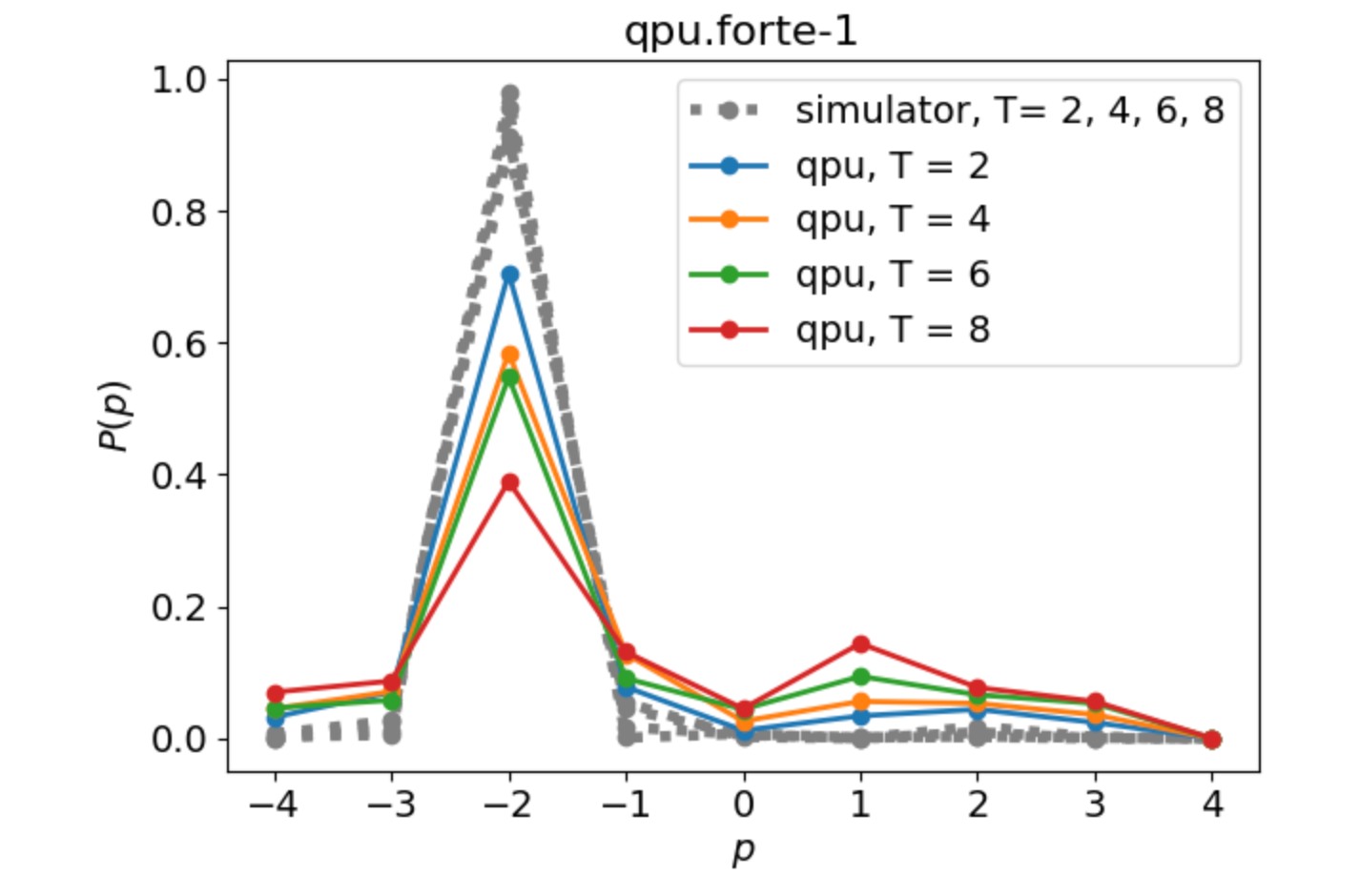
Hardware observation of dynamical localization. Momentum distribution P(p) for a 3-qubit sawtooth map initialized at p(0)=-2, shown after increasing numbers of kicks T; solid curves are IonQ Forte-1 results and dashed curves are ideal simulation.
What’s next?
Quantum maps provide a useful testbed for studying how signatures of quantum chaos interplay with real quantum hardware. Natural extensions of the case study above include leveraging hardware noise to extract a quantum Lyapunov exponent from the decay of the Loschmidt echo, probing operator spreading and information scrambling through out-of-time-order correlators (OTOCs), and moving to richer dynamics by approximating more complex maps, such as the standard map, via a high-order polynomial kicking potential. All of these will keep the same efficient “diagonal phases + QFT” model structure.
References
- Notebook on the Quantum Sawtooth map.
- Georgeot, B. and Shepelyansky, D.L., 2001. "Exponential gain in quantum computing of quantum chaos and localization". Physical Review Letters, 86(13), p.2890.
- Casati, G., Chirikov, B. V., Ford, J., & Izrailev, F. M. (1979). Stochastic behavior of a quantum pendulum under a periodic perturbation. In G. Casati & J. Ford (Eds.), Stochastic Behavior in Classical and Quantum Hamiltonian Systems (Lecture Notes in Physics, Vol. 93, pp. 334–352). Springer.
- M. D. Porter, I. Joseph, "Impact of dynamics, entanglement, and Markovian noise on the fidelity of few-qubit digital quantum simulation". Journal of Plasma Physics 91.1 (2025)
Quantum Chaos
Classical chaotic dynamics is marked by sensitivity to initial conditions: two trajectories that start arbitrarily close in phase space typically separate exponentially fast under time evolution. This exponential divergence is closely tied to mixing and rapid information spreading.
Defining quantum chaos is more subtle. In a broad sense, it refers to quantum dynamics that exhibit “chaotic” hallmarks, such as rapid information scrambling and random-matrix-like features. When a quantum system has a clear classical limit, the question becomes more specific: which dynamical signatures of classical chaos remain meaningful after quantization, and what new interference-driven phenomena appear? Quantum maps offer a particularly clean and widely used setting to explore this connection.
Quantum maps
Classical maps are discrete-time dynamical rules that update a system’s coordinates from one step to the next (e.g., x(t) → x(t+1)), Similarly, quantum maps are discrete-time quantum evolutions, often obtained by quantizing classical maps. A typical example describes free evolution periodically kicked by a position-dependent potential.
Despite their simple definition, they capture key phenomena of quantum chaos, including rapid entanglement growth and interference-driven localization, and often provide insights that carry over to more realistic systems. In 1979, Casati, Chirikov, Izrailev, and Ford identified dynamical localization in kicked chaotic systems, where quantum interference suppresses classical diffusion. In 2001, Georgeot and Shepelyansky connected such maps to quantum computing, showing exponential simulation speedups for certain cases: On a classical computer, simulating a quantum map on an n-qubit Hilbert space (N=2^n) typically means storing the full state vector of 2^n complex amplitudes and updating all of them at each step, which requires a number of operations that grows on the order of 2^n in standard state-vector simulation. On a quantum computer, the state is represented directly using only n qubits, and one map iteration can be implemented as a gate sequence whose cost scales only polynomially in n.
The canonical examples of quantum maps are already well understood, and many of their characteristic phenomena can be captured in a relatively modest Hilbert space. As a result, the exponential simulation speedup does not automatically translate into a scientific “quantum advantage” for discovering new physics in these systems. Their value today is largely practical: as controllable “toy models”, quantum maps serve as sensitive benchmarks and diagnostic probes for quantum hardware, combining rich, entangling dynamics with enough structure to implement efficiently. For example, Porter and Joseph (2025) used quantum-map simulations to connect dynamical regimes with fidelity behavior and to probe noise models on real devices.
The quantum model:
The unitary evolution of quantum maps is rather simple. The periodic kicking leads to Floquet dynamics: one period is described by a single unitary U, so after T kicks the state is
where p and q are the conjugate momentum and position operators, and the system is kicked with some potential G(q). The practical point is that the kick term is diagonal in the q-basis, while the free-evolution term is diagonal in the p-basis, and the two bases are related by a (quantum) Fourier transform. A single step therefore looks like this (starting in the p-basis):
- QFT to the q-basis.
- Apply the kick phase with G(q).
- Inverse QFT back to the p-basis.
- Apply the free (quadratic ) phase.
Leveraging Classiq’s Qmod language and Synthesis
With the Qmod language, one can naturally write the Hamiltonian evolution. For the quantum sawtooth map, G(q)~ Kq^2 is also quadratic, with some kicking magnitude K. This makes the unitary evolution implementable exactly, without Trotterization or other time-discretization approximations. Here is the Qmod code for this function:
from classiq import *
from classiq.qmod.symbolic import pi

# Build a single step function
@qfunc
def single_step(kick_mag: CReal, p: QNum):
within_apply(lambda: qft(p),
 lambda: phase(kick_mag * pi * p**2)
)
phase(-pi * p**2)
The within_apply construct handles the QFT basis change, and QNum + phase express the diagonal evolution; synthesis then produces an optimized circuit. The same structure extends to non-quadratic kicks such as polynomial approximation of sinusoidal kicked-rotor potentials.
Dynamical Localization on Real Quantum Hardware
For kicking strength 0<K<1, an initially localized momentum state first diffuses classically, but after the Heisenberg time quantum interference halts the spread and produces dynamical localization. With a finite number of qubits, localization is observable only when the localization length fits within the Hilbert-space size, imposing an upper bound on K.
Here is a model on three qubits with K=0.1, in which localization is expected to occur:
@qfunc
def main(num_kicks: CInt, p: Output[QNum[3, SIGNED, 3]]):
    allocate(p)
    p ^= -2/8
    power(num_kicks, lambda: single_step(0.1, p))
# Synthesize
qprog = synthesize(main)
Leveraging Classiq’s Execution framework to run on hardware
The code below shows how to submit a batch execution for different times T, say, on IonQ machine:
# Submit a batch execution on a QPU with 1000 shots, for different timesteps
timesteps = [2 * i for i in range(1, 5)]
backend_preferences = IonqBackendPreferences(
        backend_name="qpu.forte-1", run_via_classiq=True)
execution_prefs = ExecutionPreferences(
        backend_preferences=backend_preferences, num_shots=1000
    )
# Submit a job
with ExecutionSession(qprog, execution_prefs) as es:
job = es.submit_batch_sample([{"num_kicks": t} for t in timesteps])
job_ID = job.id
Once the job is complete, we can collect the results and plot the histogram
import matplotlib.pyplot as plt

# Collect the results when the job is completed
res = ExecutionJob.from_id(job_ID).get_batch_sample_result()

for t, r in zip(timesteps, res):
df = r.dataframe
plt.plot(df["p"]*2**3, df["probability"], "o", label=f"T={t}")
plt.legend()
The figure below shows results from executing the sawtooth-map program on IonQ’s Forte-1, compared to an ideal (noiseless) simulator. We plot the probability distribution P(p) in the momentum basis. For a 3-qubit variable (Hilbert space of size 8), the momentum levels consist of eight discrete values, {−4,−3,−2,−1,0,1,2,3}. The system is initialized in a single momentum eigenstate centered at p(0)=-2, so at T=0 the distribution is sharply localized. In the noiseless simulation (dashed gray curves), the distribution remains strongly peaked near p=-2 over multiple kicks– an instance of dynamical localization in momentum space (finite-size effects, which alter ideal localization, only become relevant at much longer times). On hardware (solid colored curves), the localization around p=-2 is still clearly visible but progressively reduced as T increases, while weight spreads to other momentum values. This gradual broadening is consistent with noise increasing with circuit depth, as larger T requires more gates, leading to increased decoherence and accumulating errors that reduce the contrast of the localized peak and enhance spreading in p-space.
Hardware observation of dynamical localization. Momentum distribution P(p) for a 3-qubit sawtooth map initialized at p(0)=-2, shown after increasing numbers of kicks T; solid curves are IonQ Forte-1 results and dashed curves are ideal simulation.
What’s next?
Quantum maps provide a useful testbed for studying how signatures of quantum chaos interplay with real quantum hardware. Natural extensions of the case study above include leveraging hardware noise to extract a quantum Lyapunov exponent from the decay of the Loschmidt echo, probing operator spreading and information scrambling through out-of-time-order correlators (OTOCs), and moving to richer dynamics by approximating more complex maps, such as the standard map, via a high-order polynomial kicking potential. All of these will keep the same efficient “diagonal phases + QFT” model structure.
References
- Notebook on the Quantum Sawtooth map.
- Georgeot, B. and Shepelyansky, D.L., 2001. "Exponential gain in quantum computing of quantum chaos and localization". Physical Review Letters, 86(13), p.2890.
- Casati, G., Chirikov, B. V., Ford, J., & Izrailev, F. M. (1979). Stochastic behavior of a quantum pendulum under a periodic perturbation. In G. Casati & J. Ford (Eds.), Stochastic Behavior in Classical and Quantum Hamiltonian Systems (Lecture Notes in Physics, Vol. 93, pp. 334–352). Springer.
- M. D. Porter, I. Joseph, "Impact of dynamics, entanglement, and Markovian noise on the fidelity of few-qubit digital quantum simulation". Journal of Plasma Physics 91.1 (2025)