


Introducing Classiq’s Fault Tolerance Engine


We recently introduced the Fault Tolerance Engine into the Classiq SDK. The engine maps a logical quantum circuit, the circuit produced by synthesizing your high-level code, onto a three-dimensional surface-code lattice and estimates the total logical error for running it on error-corrected hardware. You can use it to explore how a circuit behaves under a physical noise model and how its total logical error changes as you increase the code distance.
The following sections walk through the main stages of the Fault Tolerance Engine. If you’d prefer to jump straight into the technical workflow, head to the Fault Tolerance Engine end-to-end tutorial.
For a quick overview before diving into the details, watch Ron Cohen, Classiq’s QEC Team Lead, demonstrate the Fault Tolerance Engine in this three-minute demo.
From a Quantum Model to a Topological Program
In Classiq, you start with a quantum model: a high-level description of your algorithm. You can choose an existing algorithm or application from the Classiq Library, develop one with the help of the Classiq AI Quantum Engineer, or write the code yourself in Qmod, Classiq’s high-level quantum programming language.
Here’s a simple arithmetic example:
@qfunc
def main(
    a: Output[QNum],
    b: Output[QNum],
    c: Output[QNum],
    res: Output[QNum],
) -> None:
    a |= 2
    b |= 1
    c |= 5
    res |= (a + b + c & 15) % 8 ^ 3 & a ^ 10 == 4

qprog = synthesize(main)
%20(1).gif)
After your code is automatically synthesized by Classiq’s synthesis engine, export the resulting circuit in the Clifford+T gate set for use with the Fault Tolerance Engine:
clifford_t_qasm = export(
    qprog,
    target_language=TargetLanguage.QASM2,
    transpilation_config=FaultTolerantTranspilationConfig(
        # Note: We set the rotation approximation error to 1e-3.
        clifford_t_approximation_error=1e-3
    ),
)
Now, with the transpiled circuit in hand, we’re ready to route it:
topo_program = route_circuit(clifford_t_qasm)In the surface-code architecture used by the engine, each logical qubit is encoded in a patch of physical qubits. Interactions between patches use lattice surgery: patches merge and split over repeated error-correction cycles to implement logical quantum gates.
Routing turns the logical circuit into a concrete, fault-tolerant execution plan. It determines where and when each operation occurs on the surface-code lattice.
What Routing Produces
The interactive visualization below shows the routed program produced by the engine. Drag to rotate, scroll to zoom, and switch between the surface-code and logical views.
The plan occupies a three-dimensional lattice. Two axes describe the spatial arrangement of surface-code patches, including the logical qubits and the free space used for their interactions. The third axis represents time, measured in error-correction cycles. The visualization represents the routed operations as cubes connected by pipes, showing how surface-code patches evolve and interact over time.
T gates require special treatment. They consume magic states, auxiliary states prepared for implementing these gates. The engine schedules their preparation through a cultivation routine alongside the Clifford operations.
The output is a topological program: a complete layout of the circuit’s operations in space and time, together with summary statistics. Its spatial footprint and duration determine the resources needed to run the circuit fault-tolerantly and provide the basis for the error estimate.
Finding a good layout is a hard combinatorial problem. The engine automates this process, making it possible to route circuits far beyond what can be handled manually.
Modeling Logical Errors
Once the topological program is ready, the engine needs to know how noisy the underlying hardware is.
A physical noise model describes errors in hardware operations, including gates, measurements, and idle periods. A logical noise model describes the resulting error rates of protected operations, including Clifford and T gates, as a function of code distance.
Code distance is a measure of the code’s error protection; increasing it requires more physical qubits per patch. The logical noise model lets you examine how the error rates change with this choice.
You can choose a ready-made model from the Publicly Available Noise Models, eliminating the need to run the simulations yourself. Alternatively, you can generate a logical noise model from a custom physical noise model:
physical_noise = PhysicalNoiseModel(
    idle=[DepolarizeRule(p=1e-4)],
    clifford_1q=[DepolarizeRule(p=1e-4)],
    clifford_2q=[DepolarizeRule(p=1e-3)],
    measure={"Z": 5e-3, "X": 5e-3},
)

initialize_logical_noise("my_noise", physical_noise)
logical_noise = get_logical_noise("my_noise")
This stage is independent of the algorithm. The resulting logical noise model can be reused across quantum programs evaluated under the same physical noise assumptions and across the code distances represented in the model. This avoids having to simulate the full physical-qubit implementation of each circuit, which could involve millions of physical qubits.
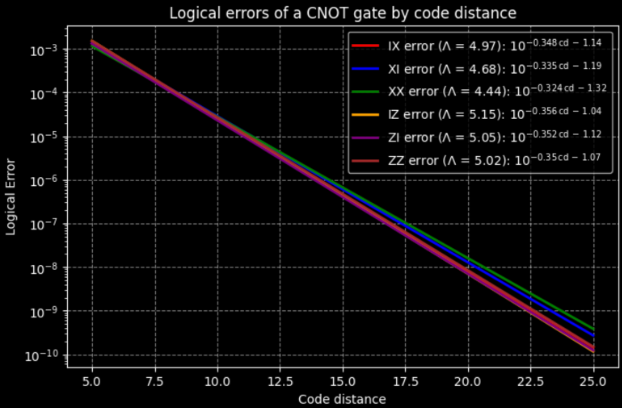
The figure below shows this relationship for a CNOT gate: as the code distance increases, the estimated logical error rates decrease rapidly across the different error channels.
Putting the Two Together
Combining the topological program with the logical noise model lets you estimate the total logical error at different code distances:
total_errors = estimate_total_errors(
    topo_program, logical_noise, code_distances
)
Here, code_distances contains the code distances you want to evaluate.
You can now move beyond asking whether an algorithm or an application is logically correct or whether its circuit can be optimized, and instead ask whether it is physically implementable on a specific machine: whether it can meet a target total logical error under that hardware’s noise model, which resources dominate its cost, and what would need to improve to make the application practical.
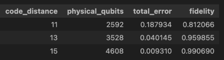
The table below shows this trade-off in practice: increasing the code distance reduces the estimated total logical error, while requiring more physical qubits.
The physical-qubit count depends on two main factors:
- The number of patches in the layout, which the router keeps tightly optimized.
- The number of physical qubits per patch, which depends directly on the code distance. Classiq’s router generates an optimized topological program that can meet a given target total logical error at a lower code distance, reducing the number of physical qubits required per patch.
Routing at Application Scale
The graphs below compare the Classiq Fault Tolerance Engine with several open-source surface-code routing approaches across two dimensions: physical-qubit footprint and routing time.
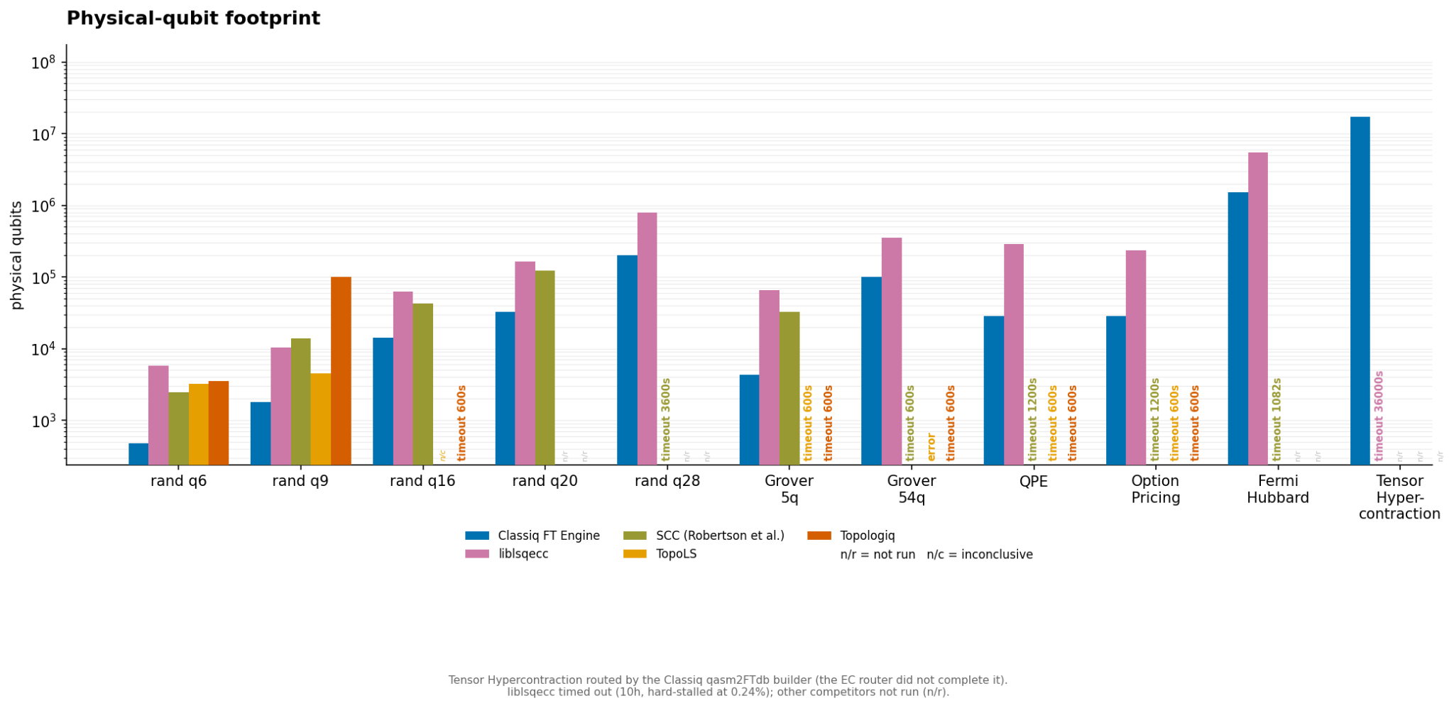
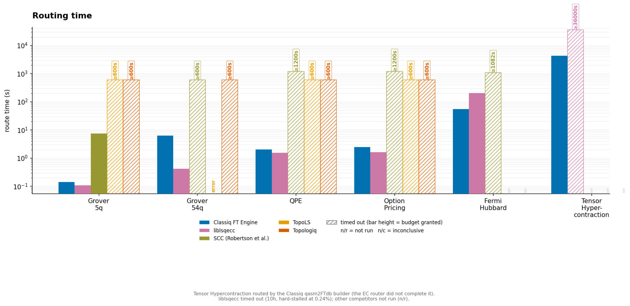
Across the workloads shown, Classiq consistently produces a smaller physical-qubit footprint than the other approaches that completed the benchmark. The Classiq Fault Tolerance Engine also completes every routing task shown within a reasonable runtime, including the larger workloads, while some other approaches do not produce results across the full benchmark set.
The tensor hypercontraction benchmark provides the clearest example of this scalability. The engine routed a circuit with approximately 219 logical qubits and 2.5–2.6 million logical gates in about one hour. Roughly half were two-qubit operations, corresponding to approximately 1.25–1.3 million routed CX interactions.
Prior work on surface-code compilation has demonstrated scalability across different dimensions, including circuit width, circuit size, and lattice-surgery and magic-state scheduling [1–7]. However, differences in compilation models, workloads, and resource assumptions make direct comparisons difficult.
We are not aware of a published, fully automatic surface-code routing result combining comparable circuit width and two-qubit interaction volume. We therefore view this result as evidence of scalability on a demanding application-level workload, rather than an absolute record across all surface-code compilation settings.
These results highlight the scalability of Classiq’s Fault Tolerance Engine and its ability to automatically route demanding, application-scale circuits.
Ready to try it yourself? Explore the Fault Tolerance Engine end-to-end tutorial to run the full workflow, or dive deeper into the Fault Tolerance and Error Correction user guides.
References
[1] A. M. Lavi et al., “Dependency-Aware Compilation for Surface Code Quantum Architectures,” Proceedings of the ACM on Programming Languages, 2025.
[2] J. Zhou, Y. Liu, E. Decker, J. Kalloor, M. Weiden, K. Chen, C. Iancu, and G. Li, “TopoLS: Lattice Surgery Compilation via Topological Program Transformations,” arXiv:2601.23109, 2026.
[3] G. Watkins, H. M. Nguyen, K. Watkins, S. Pearce, H.-K. Lau, and A. Paler, “A High Performance Compiler for Very Large Scale Surface Code Computations,” Quantum 8, 1354, 2024.
[4] S. Hofmeyr, M. Weiden, J. Kalloor, J. Kubiatowicz, and C. Iancu, “Scheduling Lattice Surgery with Magic State Cultivation,” arXiv:2512.06484, 2025.
[5] A. Silva, X. Zhang, Z. Webb, M. Kramer, C.-W. Yang, X. Liu, J. Lemieux, K.-W. Chen, A. Scherer, and P. Ronagh, “Multi-qubit Lattice Surgery Scheduling,” TQC 2024, LIPIcs 310, 1:1–1:22, 2024.
[6] J. Lee, D. W. Berry, C. Gidney, W. J. Huggins, J. R. McClean, N. Wiebe, and R. Babbush, “Even More Efficient Quantum Computations of Chemistry Through Tensor Hypercontraction,” PRX Quantum 2, 030305, 2021.
[7] R. Iacobacci, T. Hao, N. Patel, and S. Niu, “Flow-Based Lattice Surgery Optimization with Runtime T Gate Scheduling,” arXiv:2609.23756, 2026.
We recently introduced the Fault Tolerance Engine into the Classiq SDK. The engine maps a logical quantum circuit, the circuit produced by synthesizing your high-level code, onto a three-dimensional surface-code lattice and estimates the total logical error for running it on error-corrected hardware. You can use it to explore how a circuit behaves under a physical noise model and how its total logical error changes as you increase the code distance.
The following sections walk through the main stages of the Fault Tolerance Engine. If you’d prefer to jump straight into the technical workflow, head to the Fault Tolerance Engine end-to-end tutorial.
For a quick overview before diving into the details, watch Ron Cohen, Classiq’s QEC Team Lead, demonstrate the Fault Tolerance Engine in this three-minute demo.
From a Quantum Model to a Topological Program
In Classiq, you start with a quantum model: a high-level description of your algorithm. You can choose an existing algorithm or application from the Classiq Library, develop one with the help of the Classiq AI Quantum Engineer, or write the code yourself in Qmod, Classiq’s high-level quantum programming language.
Here’s a simple arithmetic example:
@qfunc
def main(
    a: Output[QNum],
    b: Output[QNum],
    c: Output[QNum],
    res: Output[QNum],
) -> None:
    a |= 2
    b |= 1
    c |= 5
    res |= (a + b + c & 15) % 8 ^ 3 & a ^ 10 == 4

qprog = synthesize(main)
After your code is automatically synthesized by Classiq’s synthesis engine, export the resulting circuit in the Clifford+T gate set for use with the Fault Tolerance Engine:
clifford_t_qasm = export(
    qprog,
    target_language=TargetLanguage.QASM2,
    transpilation_config=FaultTolerantTranspilationConfig(
        # Note: We set the rotation approximation error to 1e-3.
        clifford_t_approximation_error=1e-3
    ),
)
Now, with the transpiled circuit in hand, we’re ready to route it:
topo_program = route_circuit(clifford_t_qasm)In the surface-code architecture used by the engine, each logical qubit is encoded in a patch of physical qubits. Interactions between patches use lattice surgery: patches merge and split over repeated error-correction cycles to implement logical quantum gates.
Routing turns the logical circuit into a concrete, fault-tolerant execution plan. It determines where and when each operation occurs on the surface-code lattice.
What Routing Produces
The interactive visualization below shows the routed program produced by the engine. Drag to rotate, scroll to zoom, and switch between the surface-code and logical views.
The plan occupies a three-dimensional lattice. Two axes describe the spatial arrangement of surface-code patches, including the logical qubits and the free space used for their interactions. The third axis represents time, measured in error-correction cycles. The visualization represents the routed operations as cubes connected by pipes, showing how surface-code patches evolve and interact over time.
T gates require special treatment. They consume magic states, auxiliary states prepared for implementing these gates. The engine schedules their preparation through a cultivation routine alongside the Clifford operations.
The output is a topological program: a complete layout of the circuit’s operations in space and time, together with summary statistics. Its spatial footprint and duration determine the resources needed to run the circuit fault-tolerantly and provide the basis for the error estimate.
Finding a good layout is a hard combinatorial problem. The engine automates this process, making it possible to route circuits far beyond what can be handled manually.
Modeling Logical Errors
Once the topological program is ready, the engine needs to know how noisy the underlying hardware is.
A physical noise model describes errors in hardware operations, including gates, measurements, and idle periods. A logical noise model describes the resulting error rates of protected operations, including Clifford and T gates, as a function of code distance.
Code distance is a measure of the code’s error protection; increasing it requires more physical qubits per patch. The logical noise model lets you examine how the error rates change with this choice.
You can choose a ready-made model from the Publicly Available Noise Models, eliminating the need to run the simulations yourself. Alternatively, you can generate a logical noise model from a custom physical noise model:
physical_noise = PhysicalNoiseModel(
    idle=[DepolarizeRule(p=1e-4)],
    clifford_1q=[DepolarizeRule(p=1e-4)],
    clifford_2q=[DepolarizeRule(p=1e-3)],
    measure={"Z": 5e-3, "X": 5e-3},
)

initialize_logical_noise("my_noise", physical_noise)
logical_noise = get_logical_noise("my_noise")
This stage is independent of the algorithm. The resulting logical noise model can be reused across quantum programs evaluated under the same physical noise assumptions and across the code distances represented in the model. This avoids having to simulate the full physical-qubit implementation of each circuit, which could involve millions of physical qubits.
The figure below shows this relationship for a CNOT gate: as the code distance increases, the estimated logical error rates decrease rapidly across the different error channels.
Putting the Two Together
Combining the topological program with the logical noise model lets you estimate the total logical error at different code distances:
total_errors = estimate_total_errors(
    topo_program, logical_noise, code_distances
)
Here, code_distances contains the code distances you want to evaluate.
You can now move beyond asking whether an algorithm or an application is logically correct or whether its circuit can be optimized, and instead ask whether it is physically implementable on a specific machine: whether it can meet a target total logical error under that hardware’s noise model, which resources dominate its cost, and what would need to improve to make the application practical.
The table below shows this trade-off in practice: increasing the code distance reduces the estimated total logical error, while requiring more physical qubits.
The physical-qubit count depends on two main factors:
- The number of patches in the layout, which the router keeps tightly optimized.
- The number of physical qubits per patch, which depends directly on the code distance. Classiq’s router generates an optimized topological program that can meet a given target total logical error at a lower code distance, reducing the number of physical qubits required per patch.
Routing at Application Scale
The graphs below compare the Classiq Fault Tolerance Engine with several open-source surface-code routing approaches across two dimensions: physical-qubit footprint and routing time.
Across the workloads shown, Classiq consistently produces a smaller physical-qubit footprint than the other approaches that completed the benchmark. The Classiq Fault Tolerance Engine also completes every routing task shown within a reasonable runtime, including the larger workloads, while some other approaches do not produce results across the full benchmark set.
The tensor hypercontraction benchmark provides the clearest example of this scalability. The engine routed a circuit with approximately 219 logical qubits and 2.5–2.6 million logical gates in about one hour. Roughly half were two-qubit operations, corresponding to approximately 1.25–1.3 million routed CX interactions.
Prior work on surface-code compilation has demonstrated scalability across different dimensions, including circuit width, circuit size, and lattice-surgery and magic-state scheduling [1–7]. However, differences in compilation models, workloads, and resource assumptions make direct comparisons difficult.
We are not aware of a published, fully automatic surface-code routing result combining comparable circuit width and two-qubit interaction volume. We therefore view this result as evidence of scalability on a demanding application-level workload, rather than an absolute record across all surface-code compilation settings.
These results highlight the scalability of Classiq’s Fault Tolerance Engine and its ability to automatically route demanding, application-scale circuits.
Ready to try it yourself? Explore the Fault Tolerance Engine end-to-end tutorial to run the full workflow, or dive deeper into the Fault Tolerance and Error Correction user guides.
References
[1] A. M. Lavi et al., “Dependency-Aware Compilation for Surface Code Quantum Architectures,” Proceedings of the ACM on Programming Languages, 2025.
[2] J. Zhou, Y. Liu, E. Decker, J. Kalloor, M. Weiden, K. Chen, C. Iancu, and G. Li, “TopoLS: Lattice Surgery Compilation via Topological Program Transformations,” arXiv:2601.23109, 2026.
[3] G. Watkins, H. M. Nguyen, K. Watkins, S. Pearce, H.-K. Lau, and A. Paler, “A High Performance Compiler for Very Large Scale Surface Code Computations,” Quantum 8, 1354, 2024.
[4] S. Hofmeyr, M. Weiden, J. Kalloor, J. Kubiatowicz, and C. Iancu, “Scheduling Lattice Surgery with Magic State Cultivation,” arXiv:2512.06484, 2025.
[5] A. Silva, X. Zhang, Z. Webb, M. Kramer, C.-W. Yang, X. Liu, J. Lemieux, K.-W. Chen, A. Scherer, and P. Ronagh, “Multi-qubit Lattice Surgery Scheduling,” TQC 2024, LIPIcs 310, 1:1–1:22, 2024.
[6] J. Lee, D. W. Berry, C. Gidney, W. J. Huggins, J. R. McClean, N. Wiebe, and R. Babbush, “Even More Efficient Quantum Computations of Chemistry Through Tensor Hypercontraction,” PRX Quantum 2, 030305, 2021.
[7] R. Iacobacci, T. Hao, N. Patel, and S. Niu, “Flow-Based Lattice Surgery Optimization with Runtime T Gate Scheduling,” arXiv:2609.23756, 2026.