


Quantum Linear Solvers for CFD: From Algorithmic Promise to Practical Performance


By: Tomer Goldfriend, Classiq Technologies, Leigh Lapworth, Rolls-Royce plc
Computational Fluid Dynamics, or CFD, is one of the most demanding tasks in scientific computing. It appears in many important applications across science and engineering: from the simulation of astrophysical phenomena such as galaxy formation and supernova explosions, to flows around aircraft, and through jet engines including compressors, turbines, and combustion chambers. These simulations often require solving large, coupled systems of nonlinear equations, making CFD a major consumer of high-performance computing resources. This computational cost is one reason CFD has become a natural target for quantum algorithms, which promise speedups for various computational tasks.
One of the most promising such algorithms for CFD is the Quantum Linear Solver, or QLS for short. Given a matrix A and a vector b, the task is to find a solution vector x such that Ax=b — a type of problem that sits at the core of many CFD schemes. The hardness of the problem is characterized by two quantities: the matrix size N and its condition number κ. Consider what this means in practice: Rolls-Royce simulates the airflow inside jet engines to guide the design of its next-generation products.
The linear systems that arise in such simulations can have N and κ reaching 106 -109 or beyond — pushing the limits of the most powerful classical solvers. A QLS can, under certain conditions, efficiently encode the solution in a quantum state using only N qubits, meaning that, notionally, a modest quantum processor can represent solution vectors of exponentially large dimension relative to its classical counterpart.
Yet, quantum algorithms operate on fundamentally different principles from classical ones, and embedding a QLS into a CFD workflow is far from straightforward.
The approximate nature of quantum algorithms
When working with quantum algorithms for solving linear systems, two key challenges arise:
Readout and sampling error. The solution vector x is not directly accessible: it is encoded in the amplitudes of a quantum state, and reading it out requires repeated measurements, introducing an inherent sampling error.
Algorithmic error and circuit depth. Quantum linear solvers involve arbitrary single-qubit rotations. In the fault-tolerant regime, these must be decomposed into sequences of elementary gates (e.g., Clifford+T gates). Achieving high accuracy requires many such decompositions, making the number of single-qubit rotations a critical resource to minimize for early fault-tolerant quantum processors.
Both challenges reflect the inherently approximate nature of a QLS, in contrast to classical solvers, which are typically run until the solution converges to a specified tolerance. Designing a quantum application that manages these error sources at the algorithmic level — before any quantum error correction enters the picture — is already challenging.
Moreover, CFD solvers are nonlinear, and solving a linear system typically appears as an inner step within an iterative loop. Replacing the classical linear solver with a quantum one therefore gives rise to a hybrid classical-quantum scheme, where the approximate nature of the solver is even more pronounced: errors introduced by the quantum part at each step can potentially accumulate, degrading the convergence of the full scheme.
While theoretical error bounds exist for the various approximate components, they characterize the solver in isolation and do not tell us how errors propagate through a full hybrid application — making the actual behavior inherently problem-specific.
A practical approach
Taking a more practical approach is essential to move from theory to real-world impact. Classiq specializes in designing, compiling, and executing quantum algorithms, and Rolls-Royce is well acquainted with the demands of CFD, using large-scale simulations in the design of their jet engines.
In a recent collaboration [1], the two companies joined forces to tackle a concrete question: can a QLS be meaningfully embedded into a real CFD workflow, and what are the true costs of its approximate nature? To answer this, we embedded a QLS into a hybrid classical-quantum CFD scheme and numerically studied the interplay between algorithmic error, quantum resource requirements, and the convergence of the full CFD iteration. To isolate the different error sources, we neglected measurement errors and focused on algorithmic errors alone.
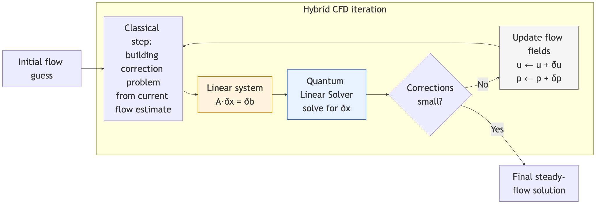
We used a CFD application made publicly available by Rolls-Royce (github.com/rolls-royce/qc-cfd). It simulates steady flow through a 1D nozzle, including transonic flow with shocks. The solver uses an outer fixed-point iteration (Figure 1): at each step, the nonlinear momentum terms are linearized around the current solution estimate, producing a linear system, i.e., of the form Ax=b, for the velocity and pressure corrections.
This system is solved, the solution is used to update the flow field, and the process repeats until convergence. It is precisely this inner linear system that we replace with a QLS. The size of the linear problem, N, corresponds to the number of mesh points, and thus to the spatial resolution at which the flow is described.
We focused on QLS algorithms based on polynomial approximation. The idea is to find a polynomial Pd of degree d that approximates the inverse function over the spectral interval of A:
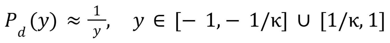
Outside this interval the polynomial can take any value. Known quantum techniques then apply this transformation to the matrix itself, giving Pd (A)≈A-1 , and acting on a quantum state encoding b yields a quantum state encoding the desired solution x. The larger the condition number , the wider the interval over which the inverse must be approximated, and therefore the higher the polynomial degree required (Fig. 2(a))— which maps directly to the circuit depth and quantum resource cost, as we describe next.
How to encode a polynomial transformation on a quantum computer?
It is useful to write the polynomial approximation as a sum of Chebyshev polynomials:
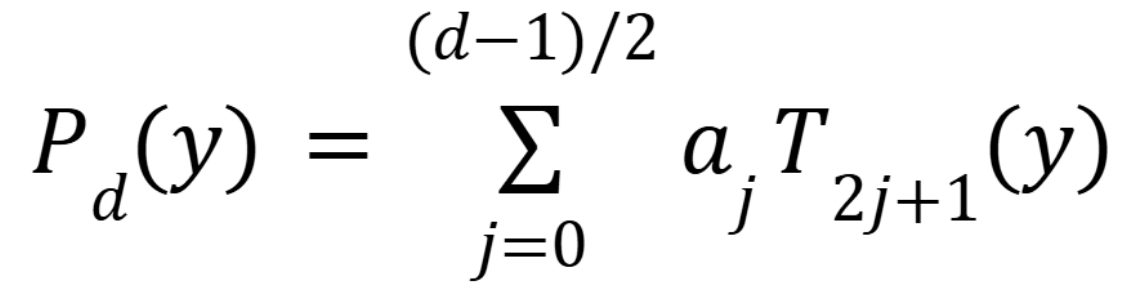
Where Ti is the Chebyshev polynomial of degree i, and the coefficients aj fully characterize the approximation. The most widely studied technique for quantum matrix inversion is the Quantum Singular Value Transformation (QSVT) approach. It is based on Quantum Signal Processing: the polynomial transformation is implemented by interleaving queries to a quantum encoding of A with single-qubit rotations on an auxiliary qubit.
The rotation angles are not the polynomial coefficients directly — they are derived from them through a classical pre-computation. For a polynomial of degree d, the number of rotations scales linearly with d — making the polynomial degree the primary lever for controlling the overall resource cost.
The quantum solver accuracy is set by the degree of the polynomial approximation: for a target error bound ε, the required degree scales as d ~ k log(k/ε). For realistic CFD problems, the condition number can reach κ>106. Matching the accuracy of classical double-precision solvers, with ε~10-12, then gives d>107. Counting only the single-qubit rotations on the QSVT auxiliary qubit (and setting aside the cost of the encoding queries) this already amounts to tens of millions of arbitrary rotations.
In the fault-tolerant setting, each of these must be decomposed into sequences of elementary gates, multiplying the cost further. It is therefore plausible that the first practically useful fault-tolerant quantum applications will need to operate with some level of algorithmic approximation, accepting a larger ε in exchange for a substantially reduced circuit cost. This is a direct manifestation of the algorithmic error challenge — and all of this is even before considering any measurement effects.
Insights from experimenting with the hybrid solver
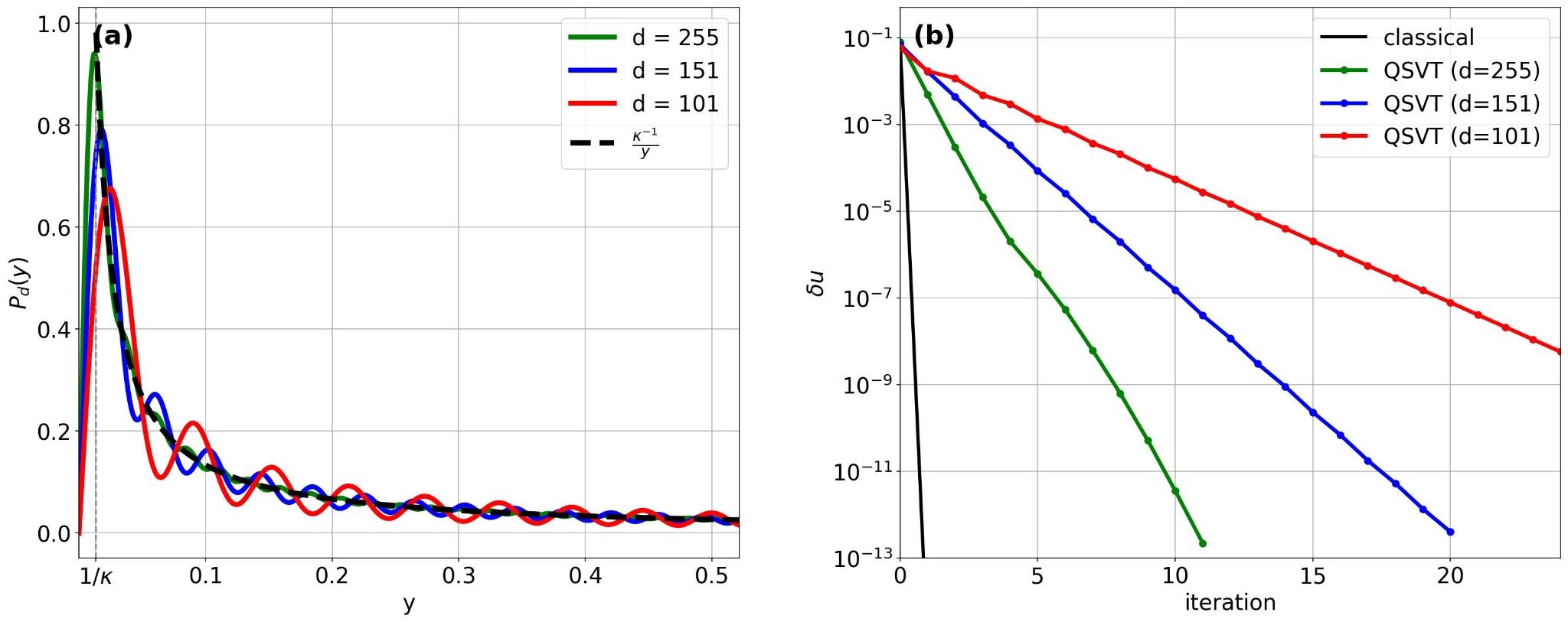
As a first step, we ran the full hybrid CFD application, plugging in the QSVT solver in place of the classical one. The problem we examined is a relatively simple one, with a condition number of κ≈100, which corresponds to a degree d≈1400 for an accuracy comparable to classical solvers. Instead of working with this theoretical bound, we chose to fix the polynomial degree and run the full CFD. As shown in Figure 2(b), lower degrees lead to more nonlinear CFD iterations, but convergence is still achieved!
The reason for this behavior becomes clear when thinking about the big picture: a CFD solver on a fixed mesh, with an inner linear solver iteratively correcting the nonlinear solution. The QLS is designed such that the polynomial Pd acts on the singular values of A: each singular value y is mapped to Pd(y)≈1/y , and the accuracy of this approximation varies across the spectral interval. Small singular values correspond to the low-frequency, long-wavelength components of the solution, while large ones correspond to high-frequency components.
With this in mind, Figure 2(a) shows that a higher polynomial degree improves the approximation in two ways: it is less oscillatory, and it remains accurate for smaller singular values. Since the CFD scheme is less sensitive to errors in the low-frequency components, a moderate polynomial degree — one that still resolves the high-frequency components accurately — is sufficient to preserve convergence.
Can we relax quantum resources further?
We learned that CFD convergence does not require an exact inverse per nonlinear iteration. Can we exploit this fact to reduce quantum resources further? The answer is yes.
We introduce a less common QLS algorithm, Chebyshev-LCU algorithm, or Cheb-LCU for short, and devise an approximate implementation of it. In this solver, the polynomial transformation is implemented by explicitly loading the polynomial coefficients {a0 , a1,...,a(d-1)/2 } onto d auxiliary qubits. Since the coefficients are in general arbitrary values, loading them requires d single-qubit rotations.
.png)
In terms of gate count, QSVT and Cheb-LCU are similar: both require d single-qubit rotations for applying a degree-d polynomial. The difference lies in how these rotations are used. In QSVT, the rotation angles are determined by a nonlinear mapping from the polynomial coefficients — an indirect encoding. In Cheb-LCU, the rotations directly load the coefficients onto the auxiliary qubits. Cheb-LCU therefore requires more qubits, but this direct encoding of the coefficients opens a natural path to approximation.
We can ask: what if we fix the polynomial degree but replace the exact coefficients with an approximated set that can be loaded more efficiently? If the coefficients admit a smooth or structured approximation, they can be represented with far fewer distinct rotation angles, directly reducing the gate count — while, as we saw, still preserving CFD convergence.
Figure 3(a) shows the Chebyshev coefficients {aj} (green dots) for a degree d=255 polynomial approximation of the inverse function. They follow a smooth, structured curve — suggesting that they can be loaded onto qubits efficiently. One option is to fit them to a simple function, such as a straight line (dashed gray curve), for which efficient quantum loading algorithms are known.
We took an even simpler approach, using an approximate state preparation technique that directly trades loading accuracy for gate count reduction. The magenta dots in Figure 3(a) show a structured, approximate version of the original coefficients that requires significantly fewer quantum resources to load. Plugging this into the Cheb-LCU solver yields an approximate Cheb-LCU algorithm, whose effect on the full CFD we then examine.
The results are shown in Figure 3(b). With an order of magnitude reduction in gate count, the CFD scheme requires roughly twice as many iterations — yet convergence is clearly preserved. This behavior can be understood in light of the insights from Figure 2: the approximate polynomial retains the main trend of the inverse function across most of the spectral interval, with deviations confined to localized regions. The broad accuracy explains why convergence is preserved; the localized inaccuracies account for the moderate slowdown.
What is next?
Quantum CFD applications do not need to wait for perfect solvers. A hybrid CFD scheme can tolerate meaningful approximation in the quantum linear solver, both from using a low-degree polynomial and from approximate coefficient loading, with only a moderate increase in iteration count. This suggests that the stringent accuracy requirements often assumed in quantum algorithm analyses may be relaxed in practice, opening a more accessible path toward the first practically useful fault-tolerant quantum applications in scientific computing.
Our study is a first step, carried out on a small-scale geometry with a modest condition number, far from the demands of industrial CFD. At this small scale, the approximate Cheb-LCU approach reduces the required single-qubit rotations by over an order of magnitude compared to QSVT, while keeping the full CFD convergence intact. How this resource reduction scales with condition number and problem size in real-world settings is an exciting open question. A natural next step is also to bring in the other approximated elements of the quantum pipeline, such as shot measurement errors and approximate data loading of the matrix A, to build a complete picture of the full error budget. We believe it is precisely this kind of end-to-end understanding — going beyond asymptotic complexity to actual behavior in a real workflow — that bridges algorithmic promise to practical performance.
References:
[1] T. Goldfriend, L. Lapworth, N. Yoran, and A. Naveh. "Approximate Quantum Linear Solvers
for Hybrid CFD: End-to-End Analysis with a Chebyshev-LCU Approach." arXiv:2606.01067 (2026).
By: Tomer Goldfriend, Classiq Technologies, Leigh Lapworth, Rolls-Royce plc
Computational Fluid Dynamics, or CFD, is one of the most demanding tasks in scientific computing. It appears in many important applications across science and engineering: from the simulation of astrophysical phenomena such as galaxy formation and supernova explosions, to flows around aircraft, and through jet engines including compressors, turbines, and combustion chambers. These simulations often require solving large, coupled systems of nonlinear equations, making CFD a major consumer of high-performance computing resources. This computational cost is one reason CFD has become a natural target for quantum algorithms, which promise speedups for various computational tasks.
One of the most promising such algorithms for CFD is the Quantum Linear Solver, or QLS for short. Given a matrix A and a vector b, the task is to find a solution vector x such that Ax=b — a type of problem that sits at the core of many CFD schemes. The hardness of the problem is characterized by two quantities: the matrix size N and its condition number κ. Consider what this means in practice: Rolls-Royce simulates the airflow inside jet engines to guide the design of its next-generation products.
The linear systems that arise in such simulations can have N and κ reaching 106 -109 or beyond — pushing the limits of the most powerful classical solvers. A QLS can, under certain conditions, efficiently encode the solution in a quantum state using only N qubits, meaning that, notionally, a modest quantum processor can represent solution vectors of exponentially large dimension relative to its classical counterpart.
Yet, quantum algorithms operate on fundamentally different principles from classical ones, and embedding a QLS into a CFD workflow is far from straightforward.
The approximate nature of quantum algorithms
When working with quantum algorithms for solving linear systems, two key challenges arise:
Readout and sampling error. The solution vector x is not directly accessible: it is encoded in the amplitudes of a quantum state, and reading it out requires repeated measurements, introducing an inherent sampling error.
Algorithmic error and circuit depth. Quantum linear solvers involve arbitrary single-qubit rotations. In the fault-tolerant regime, these must be decomposed into sequences of elementary gates (e.g., Clifford+T gates). Achieving high accuracy requires many such decompositions, making the number of single-qubit rotations a critical resource to minimize for early fault-tolerant quantum processors.
Both challenges reflect the inherently approximate nature of a QLS, in contrast to classical solvers, which are typically run until the solution converges to a specified tolerance. Designing a quantum application that manages these error sources at the algorithmic level — before any quantum error correction enters the picture — is already challenging.
Moreover, CFD solvers are nonlinear, and solving a linear system typically appears as an inner step within an iterative loop. Replacing the classical linear solver with a quantum one therefore gives rise to a hybrid classical-quantum scheme, where the approximate nature of the solver is even more pronounced: errors introduced by the quantum part at each step can potentially accumulate, degrading the convergence of the full scheme.
While theoretical error bounds exist for the various approximate components, they characterize the solver in isolation and do not tell us how errors propagate through a full hybrid application — making the actual behavior inherently problem-specific.
A practical approach
Taking a more practical approach is essential to move from theory to real-world impact. Classiq specializes in designing, compiling, and executing quantum algorithms, and Rolls-Royce is well acquainted with the demands of CFD, using large-scale simulations in the design of their jet engines.
In a recent collaboration [1], the two companies joined forces to tackle a concrete question: can a QLS be meaningfully embedded into a real CFD workflow, and what are the true costs of its approximate nature? To answer this, we embedded a QLS into a hybrid classical-quantum CFD scheme and numerically studied the interplay between algorithmic error, quantum resource requirements, and the convergence of the full CFD iteration. To isolate the different error sources, we neglected measurement errors and focused on algorithmic errors alone.
We used a CFD application made publicly available by Rolls-Royce (github.com/rolls-royce/qc-cfd). It simulates steady flow through a 1D nozzle, including transonic flow with shocks. The solver uses an outer fixed-point iteration (Figure 1): at each step, the nonlinear momentum terms are linearized around the current solution estimate, producing a linear system, i.e., of the form Ax=b, for the velocity and pressure corrections.
This system is solved, the solution is used to update the flow field, and the process repeats until convergence. It is precisely this inner linear system that we replace with a QLS. The size of the linear problem, N, corresponds to the number of mesh points, and thus to the spatial resolution at which the flow is described.
We focused on QLS algorithms based on polynomial approximation. The idea is to find a polynomial Pd of degree d that approximates the inverse function over the spectral interval of A:
Outside this interval the polynomial can take any value. Known quantum techniques then apply this transformation to the matrix itself, giving Pd (A)≈A-1 , and acting on a quantum state encoding b yields a quantum state encoding the desired solution x. The larger the condition number , the wider the interval over which the inverse must be approximated, and therefore the higher the polynomial degree required (Fig. 2(a))— which maps directly to the circuit depth and quantum resource cost, as we describe next.
How to encode a polynomial transformation on a quantum computer?
It is useful to write the polynomial approximation as a sum of Chebyshev polynomials:
Where Ti is the Chebyshev polynomial of degree i, and the coefficients aj fully characterize the approximation. The most widely studied technique for quantum matrix inversion is the Quantum Singular Value Transformation (QSVT) approach. It is based on Quantum Signal Processing: the polynomial transformation is implemented by interleaving queries to a quantum encoding of A with single-qubit rotations on an auxiliary qubit.
The rotation angles are not the polynomial coefficients directly — they are derived from them through a classical pre-computation. For a polynomial of degree d, the number of rotations scales linearly with d — making the polynomial degree the primary lever for controlling the overall resource cost.
The quantum solver accuracy is set by the degree of the polynomial approximation: for a target error bound ε, the required degree scales as d ~ k log(k/ε). For realistic CFD problems, the condition number can reach κ>106. Matching the accuracy of classical double-precision solvers, with ε~10-12, then gives d>107. Counting only the single-qubit rotations on the QSVT auxiliary qubit (and setting aside the cost of the encoding queries) this already amounts to tens of millions of arbitrary rotations.
In the fault-tolerant setting, each of these must be decomposed into sequences of elementary gates, multiplying the cost further. It is therefore plausible that the first practically useful fault-tolerant quantum applications will need to operate with some level of algorithmic approximation, accepting a larger ε in exchange for a substantially reduced circuit cost. This is a direct manifestation of the algorithmic error challenge — and all of this is even before considering any measurement effects.
Insights from experimenting with the hybrid solver
As a first step, we ran the full hybrid CFD application, plugging in the QSVT solver in place of the classical one. The problem we examined is a relatively simple one, with a condition number of κ≈100, which corresponds to a degree d≈1400 for an accuracy comparable to classical solvers. Instead of working with this theoretical bound, we chose to fix the polynomial degree and run the full CFD. As shown in Figure 2(b), lower degrees lead to more nonlinear CFD iterations, but convergence is still achieved!
The reason for this behavior becomes clear when thinking about the big picture: a CFD solver on a fixed mesh, with an inner linear solver iteratively correcting the nonlinear solution. The QLS is designed such that the polynomial Pd acts on the singular values of A: each singular value y is mapped to Pd(y)≈1/y , and the accuracy of this approximation varies across the spectral interval. Small singular values correspond to the low-frequency, long-wavelength components of the solution, while large ones correspond to high-frequency components.
With this in mind, Figure 2(a) shows that a higher polynomial degree improves the approximation in two ways: it is less oscillatory, and it remains accurate for smaller singular values. Since the CFD scheme is less sensitive to errors in the low-frequency components, a moderate polynomial degree — one that still resolves the high-frequency components accurately — is sufficient to preserve convergence.
Can we relax quantum resources further?
We learned that CFD convergence does not require an exact inverse per nonlinear iteration. Can we exploit this fact to reduce quantum resources further? The answer is yes.
We introduce a less common QLS algorithm, Chebyshev-LCU algorithm, or Cheb-LCU for short, and devise an approximate implementation of it. In this solver, the polynomial transformation is implemented by explicitly loading the polynomial coefficients {a0 , a1,...,a(d-1)/2 } onto d auxiliary qubits. Since the coefficients are in general arbitrary values, loading them requires d single-qubit rotations.
In terms of gate count, QSVT and Cheb-LCU are similar: both require d single-qubit rotations for applying a degree-d polynomial. The difference lies in how these rotations are used. In QSVT, the rotation angles are determined by a nonlinear mapping from the polynomial coefficients — an indirect encoding. In Cheb-LCU, the rotations directly load the coefficients onto the auxiliary qubits. Cheb-LCU therefore requires more qubits, but this direct encoding of the coefficients opens a natural path to approximation.
We can ask: what if we fix the polynomial degree but replace the exact coefficients with an approximated set that can be loaded more efficiently? If the coefficients admit a smooth or structured approximation, they can be represented with far fewer distinct rotation angles, directly reducing the gate count — while, as we saw, still preserving CFD convergence.
Figure 3(a) shows the Chebyshev coefficients {aj} (green dots) for a degree d=255 polynomial approximation of the inverse function. They follow a smooth, structured curve — suggesting that they can be loaded onto qubits efficiently. One option is to fit them to a simple function, such as a straight line (dashed gray curve), for which efficient quantum loading algorithms are known.
We took an even simpler approach, using an approximate state preparation technique that directly trades loading accuracy for gate count reduction. The magenta dots in Figure 3(a) show a structured, approximate version of the original coefficients that requires significantly fewer quantum resources to load. Plugging this into the Cheb-LCU solver yields an approximate Cheb-LCU algorithm, whose effect on the full CFD we then examine.
The results are shown in Figure 3(b). With an order of magnitude reduction in gate count, the CFD scheme requires roughly twice as many iterations — yet convergence is clearly preserved. This behavior can be understood in light of the insights from Figure 2: the approximate polynomial retains the main trend of the inverse function across most of the spectral interval, with deviations confined to localized regions. The broad accuracy explains why convergence is preserved; the localized inaccuracies account for the moderate slowdown.
What is next?
Quantum CFD applications do not need to wait for perfect solvers. A hybrid CFD scheme can tolerate meaningful approximation in the quantum linear solver, both from using a low-degree polynomial and from approximate coefficient loading, with only a moderate increase in iteration count. This suggests that the stringent accuracy requirements often assumed in quantum algorithm analyses may be relaxed in practice, opening a more accessible path toward the first practically useful fault-tolerant quantum applications in scientific computing.
Our study is a first step, carried out on a small-scale geometry with a modest condition number, far from the demands of industrial CFD. At this small scale, the approximate Cheb-LCU approach reduces the required single-qubit rotations by over an order of magnitude compared to QSVT, while keeping the full CFD convergence intact. How this resource reduction scales with condition number and problem size in real-world settings is an exciting open question. A natural next step is also to bring in the other approximated elements of the quantum pipeline, such as shot measurement errors and approximate data loading of the matrix A, to build a complete picture of the full error budget. We believe it is precisely this kind of end-to-end understanding — going beyond asymptotic complexity to actual behavior in a real workflow — that bridges algorithmic promise to practical performance.
References:
[1] T. Goldfriend, L. Lapworth, N. Yoran, and A. Naveh. "Approximate Quantum Linear Solvers
for Hybrid CFD: End-to-End Analysis with a Chebyshev-LCU Approach." arXiv:2606.01067 (2026).